IMDB Ratings
Analysis of movies- IMDB dataset
# Assign IMDB data to variable
movies <- read_csv(here::here("data", "movies.csv"))
Use your data import, inspection, and cleaning skills to answer the following:
- Are there any missing values (NAs)? Are all entries distinct or are there duplicate entries?
There are no missing values according to the skim function. Nevertheless, we notice some duplicate values, for example “Nightmare on Elm Street” or “Alice in Wonderland”. We have to be careful to look at more than just the title in identifying duplicates, as some movies could have the same name, but be released twice on different dates or have a different director.
# Skim IMDB data
skim(movies)| Name | movies |
| Number of rows | 2961 |
| Number of columns | 11 |
| _______________________ | |
| Column type frequency: | |
| character | 3 |
| numeric | 8 |
| ________________________ | |
| Group variables | None |
Variable type: character
| skim_variable | n_missing | complete_rate | min | max | empty | n_unique | whitespace |
|---|---|---|---|---|---|---|---|
| title | 0 | 1 | 1 | 83 | 0 | 2907 | 0 |
| genre | 0 | 1 | 5 | 11 | 0 | 17 | 0 |
| director | 0 | 1 | 3 | 32 | 0 | 1366 | 0 |
Variable type: numeric
| skim_variable | n_missing | complete_rate | mean | sd | p0 | p25 | p50 | p75 | p100 | hist |
|---|---|---|---|---|---|---|---|---|---|---|
| year | 0 | 1 | 2.00e+03 | 9.95e+00 | 1920.0 | 2.00e+03 | 2.00e+03 | 2.01e+03 | 2.02e+03 | ▁▁▁▂▇ |
| duration | 0 | 1 | 1.10e+02 | 2.22e+01 | 37.0 | 9.50e+01 | 1.06e+02 | 1.19e+02 | 3.30e+02 | ▃▇▁▁▁ |
| gross | 0 | 1 | 5.81e+07 | 7.25e+07 | 703.0 | 1.23e+07 | 3.47e+07 | 7.56e+07 | 7.61e+08 | ▇▁▁▁▁ |
| budget | 0 | 1 | 4.06e+07 | 4.37e+07 | 218.0 | 1.10e+07 | 2.60e+07 | 5.50e+07 | 3.00e+08 | ▇▂▁▁▁ |
| cast_facebook_likes | 0 | 1 | 1.24e+04 | 2.05e+04 | 0.0 | 2.24e+03 | 4.60e+03 | 1.69e+04 | 6.57e+05 | ▇▁▁▁▁ |
| votes | 0 | 1 | 1.09e+05 | 1.58e+05 | 5.0 | 1.99e+04 | 5.57e+04 | 1.33e+05 | 1.69e+06 | ▇▁▁▁▁ |
| reviews | 0 | 1 | 5.03e+02 | 4.94e+02 | 2.0 | 1.99e+02 | 3.64e+02 | 6.31e+02 | 5.31e+03 | ▇▁▁▁▁ |
| rating | 0 | 1 | 6.39e+00 | 1.05e+00 | 1.6 | 5.80e+00 | 6.50e+00 | 7.10e+00 | 9.30e+00 | ▁▁▆▇▁ |
Produce a table with the count of movies by genre, ranked in descending order
movies%>%
  count(sort = TRUE,genre)
## # A tibble: 17 × 2 ## genre n ## <chr> <int> ## 1 Comedy 848 ## 2 Action 738 ## 3 Drama 498 ## 4 Adventure 288 ## 5 Crime 202 ## 6 Biography 135 ## 7 Horror 131 ## 8 Animation 35 ## 9 Fantasy 28 ## 10 Documentary 25 ## 11 Mystery 16 ## 12 Sci-Fi 7 ## 13 Family 3 ## 14 Musical 2 ## 15 Romance 2 ## 16 Western 2 ## 17 Thriller 1Produce a table with the average gross earning and budget (
grossandbudget) by genre. Calculate a variablereturn_on_budgetwhich shows how many $ did a movie make at the box office for each $ of its budget. Ranked genres by thisreturn_on_budgetin descending order# Create table with the average gross earning and budget avg_genre = movies%>% group_by(genre) %>% summarize(avg_earning = sum(gross)/count(genre), avg_budget = sum(budget)/count(genre)) # Create 2 columns to store the average earning and budget avg_genre%>% mutate(return_on_budget = avg_earning/avg_budget) %>% # The return is just the earning/budget arrange(desc(return_on_budget))## # A tibble: 17 × 4 ## genre avg_earning avg_budget return_on_budget ## <chr> <dbl> <dbl> <dbl> ## 1 Musical 92084000 3189500 28.9 ## 2 Family 149160478. 14833333. 10.1 ## 3 Western 20821884 3465000 6.01 ## 4 Documentary 17353973. 5887852. 2.95 ## 5 Horror 37713738. 13504916. 2.79 ## 6 Fantasy 42408841. 17582143. 2.41 ## 7 Comedy 42630552. 24446319. 1.74 ## 8 Mystery 67533021. 39218750 1.72 ## 9 Animation 98433792. 61701429. 1.60 ## 10 Biography 45201805. 28543696. 1.58 ## 11 Adventure 95794257. 66290069. 1.45 ## 12 Drama 37465371. 26242933. 1.43 ## 13 Crime 37502397. 26596169. 1.41 ## 14 Romance 31264848. 25107500 1.25 ## 15 Action 86583860. 71354888. 1.21 ## 16 Sci-Fi 29788371. 27607143. 1.08 ## 17 Thriller 2468 300000 0.00823Produce a table that shows the top 15 directors who have created the highest gross revenue in the box office. Don’t just show the total gross amount, but also the mean, median, and standard deviation per director.
# Calculate summary statistics for top 15 directors
Top_directors = movies%>%
  group_by(director) %>%
  summarise(sum_gross = sum(gross),
            mean_gross = mean(gross),
            median_gross = median(gross),
            SD_gross = sd(gross))
# Choose the top 15 with highest gross earnings
Top_directors%>%
  slice_max(sum_gross,n = 15)
## # A tibble: 15 × 5 ## director sum_gross mean_gross median_gross SD_gross ## <chr> <dbl> <dbl> <dbl> <dbl> ## 1 Steven Spielberg 4014061704 174524422. 164435221 101421051. ## 2 Michael Bay 2231242537 171634041. 138396624 127161579. ## 3 Tim Burton 2071275480 129454718. 76519172 108726924. ## 4 Sam Raimi 2014600898 201460090. 234903076 162126632. ## 5 James Cameron 1909725910 318287652. 175562880. 309171337. ## 6 Christopher Nolan 1813227576 226653447 196667606. 187224133. ## 7 George Lucas 1741418480 348283696 380262555 146193880. ## 8 Robert Zemeckis 1619309108 124562239. 100853835 91300279. ## 9 Clint Eastwood 1378321100 72543216. 46700000 75487408. ## 10 Francis Lawrence 1358501971 271700394. 281666058 135437020. ## 11 Ron Howard 1335988092 111332341 101587923 81933761. ## 12 Gore Verbinski 1329600995 189942999. 123207194 154473822. ## 13 Andrew Adamson 1137446920 284361730 279680930. 120895765. ## 14 Shawn Levy 1129750988 102704635. 85463309 65484773. ## 15 Ridley Scott 1128857598 80632686. 47775715 68812285.Finally, ratings. Produce a table that describes how ratings are distributed by genre. We don’t want just the mean, but also, min, max, median, SD and some kind of a histogram or density graph that visually shows how ratings are distributed.
# Calculate summary statistics for ratings by genre
Ratings_genre = movies%>%
  group_by(genre)%>%
  summarise(mean_ratings = mean(rating),
            min_rating = min(rating),
            max_rating = max(rating),
            median_rating = median(rating),
            SD_rating = sd(rating))
Ratings_genre
## # A tibble: 17 × 6 ## genre mean_ratings min_rating max_rating median_rating SD_rating ## <chr> <dbl> <dbl> <dbl> <dbl> <dbl> ## 1 Action 6.23 2.1 9 6.3 1.03 ## 2 Adventure 6.51 2.3 8.6 6.6 1.09 ## 3 Animation 6.65 4.5 8 6.9 0.968 ## 4 Biography 7.11 4.5 8.9 7.2 0.760 ## 5 Comedy 6.11 1.9 8.8 6.2 1.02 ## 6 Crime 6.92 4.8 9.3 6.9 0.849 ## 7 Documentary 6.66 1.6 8.5 7.4 1.77 ## 8 Drama 6.73 2.1 8.8 6.8 0.917 ## 9 Family 6.5 5.7 7.9 5.9 1.22 ## 10 Fantasy 6.15 4.3 7.9 6.45 0.959 ## 11 Horror 5.83 3.6 8.5 5.9 1.01 ## 12 Musical 6.75 6.3 7.2 6.75 0.636 ## 13 Mystery 6.86 4.6 8.5 6.9 0.882 ## 14 Romance 6.65 6.2 7.1 6.65 0.636 ## 15 Sci-Fi 6.66 5 8.2 6.4 1.09 ## 16 Thriller 4.8 4.8 4.8 4.8 NA ## 17 Western 5.7 4.1 7.3 5.7 2.26# Plot ratings by genre ggplot(movies,aes(x=rating)) + geom_density() + labs(title="There are few completely unpopular movies with a rating of less than 5",subtitle = "Density plot of movie ratings on IMDB",x = "Rating", y = "Density")+ theme_bw()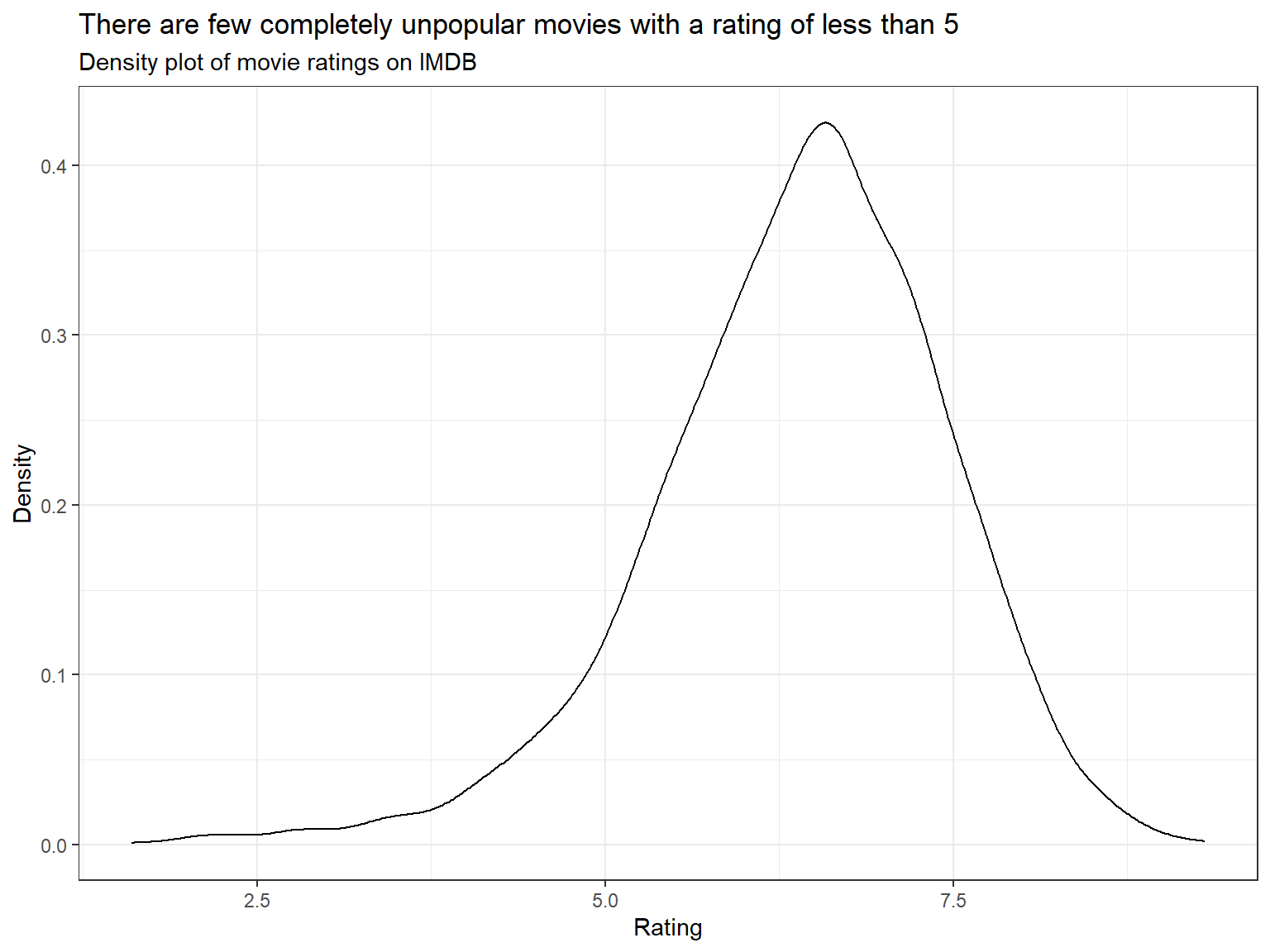
Use ggplot to answer the following
- Examine the relationship between
grossandcast_facebook_likes. Produce a scatterplot and write one sentence discussing whether the number of facebook likes that the cast has received is likely to be a good predictor of how much money a movie will make at the box office. What variable are you going to map to the Y- and X- axes?
While there seems to be a minor correlation between the amount of cast facebook likes and the money a movie makes, the relationship is not strong enough to make it a good predictor of a movie’s success.
# Map revenue vs Facebook likes
movies%>%
ggplot(aes(x=cast_facebook_likes, y = gross)) +
  geom_point()+scale_x_log10()+geom_smooth(method = "lm", se = FALSE) +
  labs(title="Cast Facebook likes do not seem to be a reliable predictor of movie success",subtitle = "Scatterplot of number of cast facebook likes and movie gross revenue",x = "Number of Cast Facebook Likes", y = "Gross Revenue")+
  theme_bw()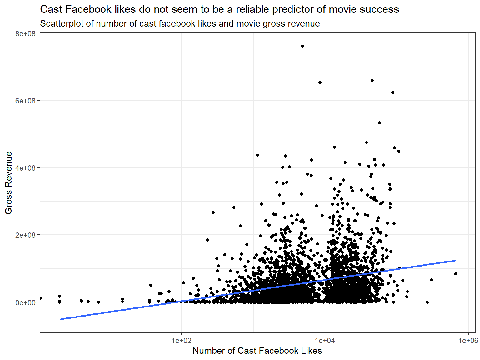
- Examine the relationship between
grossandbudget. Produce a scatterplot and write one sentence discussing whether budget is likely to be a good predictor of how much money a movie will make at the box office.
While a budget is surely not a guarantor of movie success , the fitted line has a positive slope and therefore implies that with rising budget comes rising gross revenue.
 #Map revenue vs budget
movies%>%
  ggplot(aes(x=budget,y=gross))+
  geom_point()+geom_smooth(method = "lm", se = FALSE) +
  labs(title="A higher budget seems to positively affect movie gross revenue",subtitle = "Scatterplot of movie budget and movie gross revenue",x = "Budget", y = "Gross Revenue")+
  theme_bw()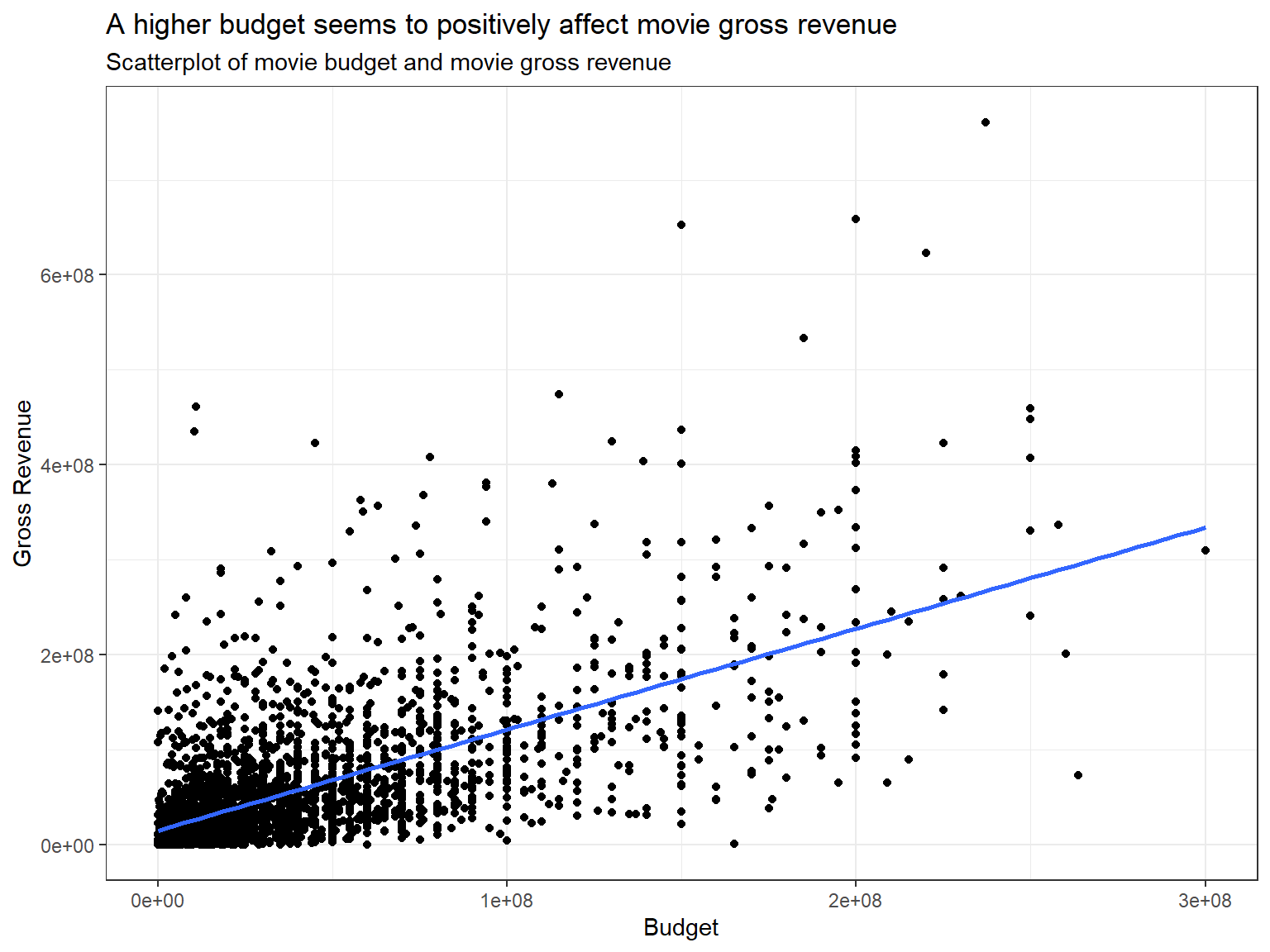
- Examine the relationship between
grossandrating. Produce a scatterplot, faceted bygenreand discuss whether IMDB ratings are likely to be a good predictor of how much money a movie will make at the box office. Is there anything strange in this dataset?
Generally, higher ratings indicates higher gross earnings for all genres for which we have a significant amount of data. However, we can also see that it is possible for movies to have a good rating while not making a lot of money. This most likely concern the likes of indie movies, that receive strong support but never make it into the pop culture.
There are some interesting anomalies in the data in the form of extreme values. Drama movies usually fall within the same range of gross revenues, however “Titanic” by James Cameron reports much higher values than the rest. Coincidentally, James Cameron is also the director for highest grossing movie in the data “Avatar”. It is also noticeable that there are no observable outliers for genres like comedy or adventure, even though there are several movies of the genre in the data. Apparently these categories do not display the required parameters to polarize the nation.
# Map revenue vs rating, faceted by genre
movies%>%
  ggplot(aes(x=rating, y = gross,color=genre))+
  geom_point()+facet_wrap(~genre)+
  labs(title="A higher rating seems to be correlated to higher gross revenues",subtitle = "Faceted scatterplot of IMDB rating and movie gross revenue",x = "IMDB Rating", y = "Gross Revenue")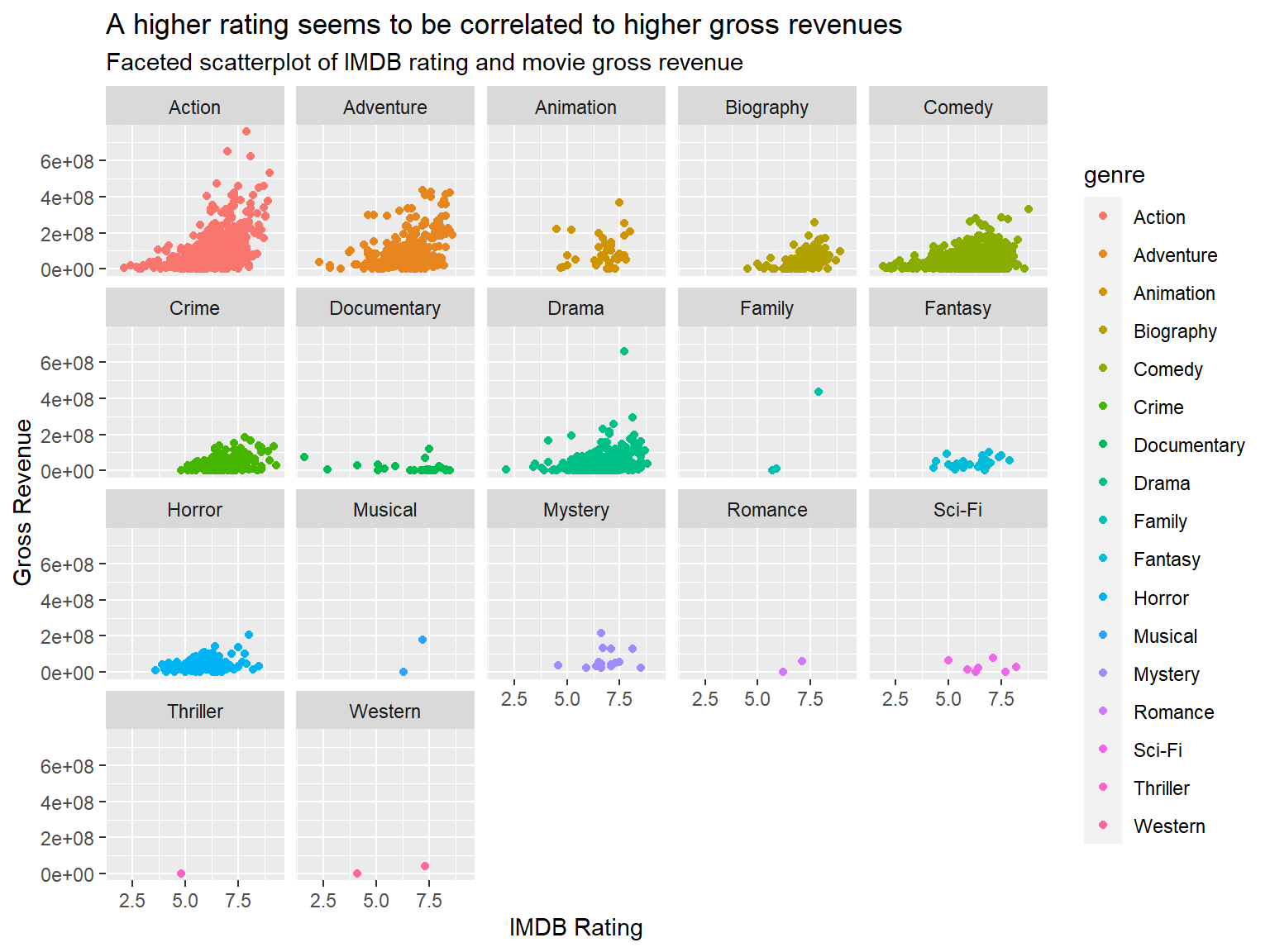
IMDB ratings: Differences between directors
Recall the IMBD ratings data. I would like you to explore whether the mean IMDB rating for Steven Spielberg and Tim Burton are the same or not. I have already calculated the confidence intervals for the mean ratings of these two directors and as you can see they overlap.
First, I would like you to reproduce this graph. You may find geom_errorbar() and geom_rect() useful.
In addition, you will run a hypothesis test. You should use both the t.test command and the infer package to simulate from a null distribution, where you assume zero difference between the two.
Before anything, write down the null and alternative hypotheses, as well as the resulting test statistic and the associated t-stat or p-value. At the end of the day, what do you conclude?
H0 = There is no difference in the average IMDB rating of Tim Burton and Steven Spielberg movies H1 = There is a difference in the average IMDB rating of Tim Burton and Steven Spielberg movies
You can load the data and examine its structure
# Load and glimpse movie data
movies <- read_csv(here::here("data", "movies.csv"))
glimpse(movies)
## Rows: 2,961
## Columns: 11
## $ title <chr> "Avatar", "Titanic", "Jurassic World", "The Avenge…
## $ genre <chr> "Action", "Drama", "Action", "Action", "Action", "…
## $ director <chr> "James Cameron", "James Cameron", "Colin Trevorrow…
## $ year <dbl> 2009, 1997, 2015, 2012, 2008, 1999, 1977, 2015, 20…
## $ duration <dbl> 178, 194, 124, 173, 152, 136, 125, 141, 164, 93, 1…
## $ gross <dbl> 7.61e+08, 6.59e+08, 6.52e+08, 6.23e+08, 5.33e+08, …
## $ budget <dbl> 2.37e+08, 2.00e+08, 1.50e+08, 2.20e+08, 1.85e+08, …
## $ cast_facebook_likes <dbl> 4834, 45223, 8458, 87697, 57802, 37723, 13485, 920…
## $ votes <dbl> 886204, 793059, 418214, 995415, 1676169, 534658, 9…
## $ reviews <dbl> 3777, 2843, 1934, 2425, 5312, 3917, 1752, 1752, 35…
## $ rating <dbl> 7.9, 7.7, 7.0, 8.1, 9.0, 6.5, 8.7, 7.5, 8.5, 7.2, …# Create list to filter for directors of interest
direc <- c("Tim Burton","Steven Spielberg")
library(ggrepel)
movies %>%
# filter and group for directors
filter(director %in% direc) %>%
group_by(director) %>%
# Calculate summary statistics
summarize(mean_rating = mean(rating),
sd_rating = sd(rating),
count = n(),
t_critical = qt(0.975, count-1)) %>%
mutate(x_min = mean_rating - t_critical*sd_rating/sqrt(count),
x_max = mean_rating + t_critical*sd_rating/sqrt(count) ) %>%
# Create confidence interval plot for directors
ggplot(aes(x = mean_rating,y=director, colour = director,
label = round(mean_rating,2), size = 10))+
geom_pointrange(aes(xmin=x_min,xmax=x_max),size=1)+
geom_errorbar(aes(xmin = x_min, xmax = x_max),
width = 0.1, size = 1.2) +
# Creating grey angle to mark overlap between intervals
geom_rect(aes(xmin = x_min[1], xmax = x_max[2],
ymin = 0, ymax = 3),
alpha = 1/8,color = NA) +
# Add labels of margins of the confidence intervals
geom_text(aes(label = round(x_min,2), x=x_min),
vjust = -1, size = 3.5,
color = "black") +
geom_text(aes(label = round(x_max,2), x=x_max),
vjust = -1, size = 3.5,
color = "black") +
geom_text(aes(label = round(mean_rating,2), x=mean_rating),
vjust = -1, size = 5,
color = "black") +
# Format plot
scale_y_discrete(limits = c("Tim Burton","Steven Spielberg"))+
theme_bw()+
theme(legend.position = "none")+
labs(title = "Do Spielberg and Burton have the same mean IMDB ratings?",
subtitle = "95% confidence intervals overlap",
x = "Mean IMDB Rating",
y = NULL) +
theme(plot.title = element_text(face="bold"))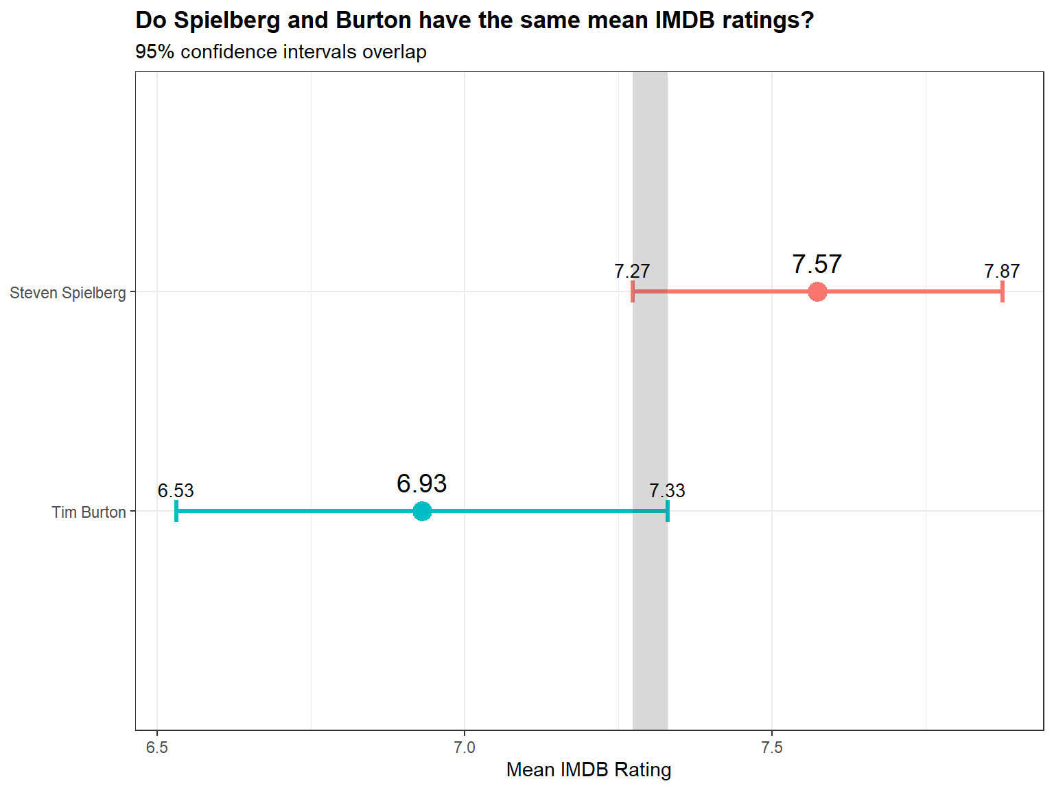
direc_data <- movies %>%
  filter(director %in% direc) %>%
  group_by(director) %>%
  summarize(rating, n = n())

# Run t-test
t.test(rating ~ director, data = direc_data )
##
## Welch Two Sample t-test
##
## data: rating by director
## t = 3, df = 31, p-value = 0.01
## alternative hypothesis: true difference in means between group Steven Spielberg and group Tim Burton is not equal to 0
## 95 percent confidence interval:
## 0.16 1.13
## sample estimates:
## mean in group Steven Spielberg mean in group Tim Burton
## 7.57 6.93As we can see from the two sample t-test, we reject the null hypothesis as 0 does not lie within the confidence interval. We can therefore say with 95% confidence that there is a signifcant difference in the average rating of Steven Spielberg and Tim Burton films. The graph confirms this, as we see only a very small and seemingly insignificant overlap between the confidence intervals. Specifically, we also see that the difference stems from Steven Spielberg having a higher average rating. Nevertheless, it should be mentioned that the sample size for both directors is rather low, with a correspondingly high t_critical. As more movies come out and the ratings do not drastically deviate from the current average, we might expect to not see any more overlap of the confidence intervals in the future.
Personally, we enjoy Beetlejuice just as much as Jurassic Park.